Multi Source BFS

In normal BFS, there is a single starting node (or source) which is pushed inside the queue from where we start traversing other nodes until the queue is not empty. Whereas in multi source BFS, we have multiple starting nodes, all of which are initially pushed into the queue and then traversal is started.

Let us consider an example of normal BFS

Given above graph, we have to find the distance between source node 1 and destination node 4.

Here's the simple BFS solution that works in O(n) time.

    #include<bits/stdc++.h>

    using namespace std;

    int distBetween(vector<int>*adj,int n,int src,int dest){

        queue<pair<int,int>>q;

        int d=0;

        q.push({src,d});

        vector<int>vis(n+1);

        while(!q.empty()){

            src=q.front().first;

            d=q.front().second;

            q.pop();

            if(vis[src])continue;

            vis[src]=1;

            if(src==dest)return d;

            for(auto &v:adj[src])

                q.push({v,d+1});

        }

        return -1;

    }

    int main(){

        system("CLS");

        int n=6;

        vector<int>adj[n+1];

        adj[1]={3,5};

        adj[2]={3,6};

        adj[3]={1,2,4,5,6};

        adj[4]={3,6};

        adj[5]={1,3,6};

        adj[6]={2,3,4,5};

        int src=1, dest=6;

        cout<<distBetween(adj,n,src,dest);

        return 0;

    };

Now, let consider a new problem. Among the nodes 1, 3 and 5, what is the closest distance from node 2?

Naive solution to this problem is to use a BFS for each given source nodes and find distance of them from destination node and return the minimum distance.

Time complexity will be O(number of nodes * BFS time for each node)

In worst case, number of nodes can be n (where n is the number of nodes in the graph), in this case time complexity will be O(n*n).

    #include<bits/stdc++.h>

    using namespace std;

    int distBetween(vector<int>*adj,int n,int src,int dest){

        queue<pair<int,int>>q;

        int d=0;

        q.push({src,d});

        vector<int>vis(n+1);

        while(!q.empty()){

            src=q.front().first;

            d=q.front().second;

            q.pop();

            if(vis[src])continue;

            vis[src]=1;

            if(src==dest)

                return d;

            for(auto &v:adj[src])

                q.push({v,d+1});

        }

        return -1;

    }

    int main(){

        system("CLS");

        int n=6;

        vector<int>adj[n+1];

        adj[1]={3,5};

        adj[2]={3,6};

        adj[3]={1,2,4,5,6};

        adj[4]={3,6};

        adj[5]={1,3,6};

        adj[6]={2,3,4,5};

        int src1=1,src2=3,src3=5, dest=6;

        cout<<min({distBetween(adj,n,src1,dest),

                   distBetween(adj,n,src2,dest),

                   distBetween(adj,n,src3,dest)});

        return 0;

    };

Efficient solution: Using multi source BFS.

It is similar to normal BFS, but unlike normal BFS, we push all the source nodes to the queue before starting the traversal.

Time complexity: O(n)

    #include<bits/stdc++.h>

    using namespace std;

    int distBetween(vector<int>*adj,int n,vector<int>&src,int dest){

       

        queue<pair<int,int>>q;

        int d=0;

        for(auto &s:src)

            q.push({s,d});

        vector<int>vis(n+1);

        while(!q.empty()){

            int s=q.front().first;

            d=q.front().second;

            q.pop();

            if(vis[s])continue;

            vis[s]=1;

            if(s==dest)

                return d;

            for(auto &v:adj[s])

                q.push({v,d+1});

        }

        return -1;

    }

    int main(){

        system("CLS");

        int n=6;

        vector<int>adj[n+1];

        adj[1]={3,5};

        adj[2]={3,6};

        adj[3]={1,2,4,5,6};

        adj[4]={3,6};

        adj[5]={1,3,6};

        adj[6]={2,3,4,5};

        int dest=6;

        vector<int>src={1,2,3};

        cout<<distBetween(adj,n,src,dest);

        return 0;

    };

---

Related problems

1. 01 Matrix

2.Distance of nearest cell having 1

3.As Far from Land as Possible

CSES Tree Algorithms: 2. Maximum Matching

CSES Tree Algorithms

2. Maximum Matching

link

CSES Tree Algorithms : 1. Subordinates

CSES Tree Algorithms

1. Subordinates

link

Flood Fill Algorithm

 Flood Fill Algorithm

Flood fill algorithm helps in visiting each and every point in a given area. It determines the area connected to a given cell in a multi-dimensional array. Following are some famous implementations of flood fill algorithm:

Bucket Fill in Paint:
Clicking in an area with this tool selected fills that area with the selected color.

Solving a Maze:
Given a matrix with some starting point, and some destination with some obstacles in between, this algorithm helps to find out the path from source to destination

Minesweeper:
When a blank cell is discovered, this algorithm helps in revealing neighboring cells. This step is done recursively till cells having numbers are discovered.

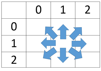
Flood fill algorithm can be simply modeled as graph traversal problem, representing the given area as a matrix and considering every cell of that matrix as a vertex that is connected to points above it, below it, to right of it, and to left of it and in case of 8-connections, to the points at both diagonals also. For example, consider the image given below.

It clearly shows how the cell in the middle is connected to cells around it. For instance, there are 8-connections like there are in Minesweeper (clicking on any cell that turns out to be blank reveals 8 cells around it which contains a number or are blank). The cell (1,1) is connected in (2,1), (1,2), (1,0), (0,0), (0,2), (2,0), (2,2) and (0,1). 

ie Each (x,y) cell is connected to (x-1,y), (x+1,y), (x,y+1), (x,y-1), (x+1,y+1), (x+1,y-1), (x-1,y+1) and (x-1,y-1).

Algorithm

function DFS(x, y, visited, n, m)
    if (x ≥ n OR y ≥ m)
        return
    if(x < 0 OR y < 0)
        return
    if(visisted[x][y] == True)
        return
    visited[x][y] = True
    DFS(x-1, y-1, visited, n, m)
    DFS(x-1, y, visited, n, m)
    DFS(x-1, y+1, visited, n, m)
    DFS(x, y-1, visited, n, m)
    DFS(x, y+1, visited, n, m)
    DFS(x+1, y-1, visited, n, m)
    DFS(x+1, y, visited, n, m)
    DFS(x+1, y+1, visited, n, m)

The above code visits each and every cell of a matrix of size $n\times m$ starting with some source cell. Time Complexity of above algorithm is O(m*n).

Click here to see the demonstration of Flood Fill Algorithm

HeapSort as a combine subroutine of MergeSort

This article is taken from my ResearchGate profile. Link . This article is under Creative Commons Licence By (cc-by).

Divide and Conquer Algorithm for Linear Search

Divide and Conquer Algorithm for Linear Search

We have seen the Binary Search Algorithm which searches for an element in a sorted array in logarithmic time. Time complexity associated with it is . 

Recurrence relation of Binary Search: 

Using the same principle of Divide, Conquer, and Combine, we can also utilize this algorithm to find an element in an unsorted array, though the time complexity will be linear .

Recurrence relation of Linear Search: 

#include<iostream>

#include<vector>

using namespace std;

int linear_search(vector<int>&v,int s,int e,int x)

{

    if(s>e)return -1;

    int m=s+(e-s)/2;

    if(v[m]==x)return m;

    int left=linear_search(v,s,m-1,x);

    int right=linear_search(v,m+1,e,x);

    if(left==-1 && right==-1)return -1;

    if(left!=-1)return left;

    else if(right!=-1)return right;

}

int main()

{

    vector<int>v={4,2,6,8,1,2,9,4};

    cout<<linear_search(v,0,v.size()-1,8);

    return 0;

}

Output: 3

Analysis of time complexity:

Sum of an array using Divide and Conquer algorithm

Sum of an array using Divide and Conquer algorithm (DAC)

Finding sum of an array is a very easy task, just add all the elements in a single pass! Time and space complexity associated with this approach is linear and constant respectively. 

In this post, I will show how we can find the sum of an array using Divide and Conquer algorithm.

First of all I would like you to have a glance at What a Divide and Conquer algorithm is? 

Divide and Conquer is an algorithmic strategy used to find solution of a particular problem by recursively breaking down the problem into sub-problems of same type, and when the base condition of the recursion is hit, assemble the results of those sub-problems to form the solution of the original problem.

This strategy often brings considerable optimizations in some while solving some problems. Some popular algorithms that implements Divide and Conquer are:

1. Quicksort

2. Mergesort

3. Binary Exponentiation

4. Quickselect

5. Straseen's algorithm (Matrix Multiplication)

6. Binary Search

The Divide and Conquer strategy can be divided into three parts:

1. Divide: Divide the larger problem into smaller sub-problems of same type.

2. Conquer: Solve the sub-problems by recursively calling until solved.

3. Combine:  Combine the sub-problems to get the final solution of the whole problem.

It becomes very easy to find the time complexity of DAC algorithms using Master Theorem.

Image given below shows how to solve recurrence relations using Master Method.

Now, coming back to the question. We have to find the sum of an array using    DAC. 

Let's formulate the solution:

Sum of an array can be found using breaking the array into two halves, add them and return the sum. Recursively break down the problem into two halves, we the array size becomes 1, return the value of that single element. So simple! 

int sum(int arr[],int start,int end)

{

    if(start==end)

    return arr[start];

    int mid=start+(end-start)/2;

    int left=sum(arr,start,mid);

    int right=sum(arr,mid+1,end);

    return left+right;

}

    int arr[]={1,2,3,-1,4,5,6,7};

    cout<<sum(arr,0,sizeof(arr)/sizeof(int)-1);

output: 27

I have traced the algorithm:

Now, let's find the time complexity of this algorithm. 

Hence, the time complexity is .

The QuickSelect Algorithm

What is QuickSelect Algorithm?

Suppose I give you an array of numbers and ask you to give me the  smallest number. How will you come out with solution?

One simple solution is to sort the array and return the element at   index, or  ARR[K-1]. 

C++ code

int kthSmallest(int *arr,int n,int k)

{

    sort(arr,arr+n);

    return arr[k-1];

}

The time complexity of this approach will be depending upon the sorting algorithm we use. Let us suppose we use the very popular comparison based sorting algorithm known as quicksort. 

Since time complexity of quicksort is  .  Therefore our naive solution will also have the same complexity of  . 

Is it a good approach?

Surely no because by sorting the whole array, we will be in the position to answer each element from k=1 to k=N ( N is the length of the array). What I want to say is we are doing extra efforts, which we can skip.

Before heading towards our goal, first let us know about the partitioning algorithm.

Partitioning Algorithm

Partitioning algorithm is a subroutine of quicksort algorithm which creates a pivot in the array and returns its index. Elements in the left hand side of the array are less than the pivot and that of right side are greater than the pivot.

for example, if the array is 3,2,1,5,6,4. Then after partitioning it will look like  1,2,3,5,6,4. 

It takes the first element and places it at some index such that all elements before it are lesser than it and all element to its right are greater than it. 

Here 3 is selected as pivot and placed at index 2. 

C++ code

int partition(int *arr,int lb,int ub)

{

    int start=lb,end=ub;

    int pivot=arr[start];

    while(start<end )

    {

        while(arr[start]<=pivot)

        ++start;

        while(arr[end]>pivot)

        --end;

        if(start<end)

        swap(arr[start],arr[end]);

    }

    swap(arr[lb],arr[end]);

    return end;

}

    

Time complexity of this partitioning algorithm is . 

QuickSelect Algorithm:

Similar to quicksort algorithm, quickselect calls partition function as it subroutine. The partition function partitions the array into two parts and returns the index of  the pivot element. 

Now, if the index of the pivot element is equal to k, then the quickselect functions returns the pivot, else if k is greater than the pivot index, then the quickselect is called for the right side of the array or if k is less than the pivot index, then the quickseleck is called for the left side of the array.

Look at the code for better understanding.

int quickSelect(int *arr,int start,int end,int k)

{

    if(start>end)

    return 0;

    int pInd=partition(arr,start,end);

    if(pInd==k)

    return arr[pInd];

    if(k>pInd)

    {  

        quickSelect(arr,pInd+1,end,k);

    }

    else

    {  

        quickSelect(arr,start,pInd-1,k);

    }

}

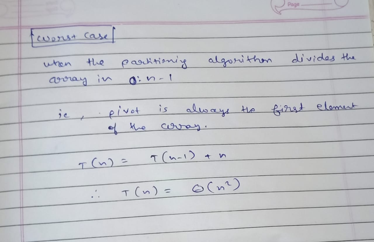
Now let's do the analysis of QuickSelect algorithm: